ctioga2 the polymorphic plotting program

Complex layouts

This page shows you how it is easy to change the layout of plots, starting from the size to insets and complex grid layouts.

Plot size

By default, ctioga2 produces a square plot of exactly 12cm by 12cm. This can be changed using the --page-size command (or -r for short):

ctioga2 -X --math 'sin(x)' --page-size '7cmx12cm'

Copy to terminal

The plots generated in this documentation have a -r 9cmx6cm transparently prepended to the commands in order to get a rectangular output.

Insets

ctioga2 supports insets, just like the old ctioga did. Only, the inset specifications are slightly different than before. See:

ctioga2 -X --math 'x**2' --inset 'tl:0.2,0.8:0.4,0.3' \
	'cos(x)' -t 'Inset !' --end 'x'

Copy to terminal

The tl:0.2,0.8:0.4,0.3 bit signifies: place the inset’s top left (tl) at the position X = 0.2, Y = 0.8 (frame positions: 0 is left or bottom, 1 is top or right), and make it 0.4 in width and 0.3 in height. See how the --end command switches back to the main plot, and how the --title command applies to the inset.

Grids

ctioga featured a way to arrange plots as “grids”. It was neither easy to use nor very satisfying. ctioga2 provides a completely different way to handle the things, through the command --setup-grid. See:

ctioga2 -X --math --setup-grid 2x2 /top 5mm \
	--inset grid:0,0 'sin(x)' \
	--next-inset grid:0,1 'x**2' \
	--next-inset grid:1,1 'x**3'

Copy to terminal

Once --setup-grid has been used, start the first plot with --inset and the next ones with --next-inset. --setup-grid takes many options to control which space should be left on the sides of the whole plot (left, top, bottom and right) and how much space should be inserted between the individual “insets” (dx, dy).

A grid element can span several rows and/or columns. Just indicate them using a range such as 0-1 instead of the column/row position:

ctioga2 -X --math --setup-grid 2x2 /top 5mm \
	--inset grid:0-1,0 'sin(x)' \
	--next-inset grid:0,1 'x**2' \
	--next-inset grid:1,1 'x**3'

Copy to terminal

A full example of a complex grid

Let’s say we want to plot sin(omega(t) t) for omega(t) that first increases linearly and then decreases symetrically back to the initial value. We want to plot the value of omega(t) above the main plot, but smaller. This is how it looks:

ruby
def omega(t)
  if t > 10
    return 3 - 0.2*(t - 10)
  else
    return 1 + 0.2 * t
  end
end
ruby end

xr = -1:21

math /xrange 0:20 /samples=1000
setup-grid 1x1,2 /top=1mm /right=2mm /dy=2mm
inset grid:0,0
  plot 'omega(x)'
  ylabel '$\omega(t)$'
  no-xlabel
  bottom ticks
  margin 0.08
  xrange $(xr)
next-inset grid:0,1
  plot 'sin(omega(x) * x)'
  ylabel '$\sin \left\{\omega(t) \, t\right\}$'
  xlabel '$t$'
  margin 0.03
  xrange $(xr)
end

Download command file

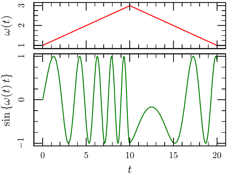
To ensure both grids have the same x range, despite the fact that we use different margin inside, we define a xr variable that holds the range and use if with xrange. To have the top and bottom plots of different size, we used 1x1,2 as an argument to setup-grid, which means that there is one column and two rows, the second being twice as large as the first (we could also have used 1x10,20, the measures a relative). We used bottom ticks to deactivate the display of tick labels on the bottom axis in the top plot. Finally, we used an inline bit of ruby code to ease the definition of omega(t).

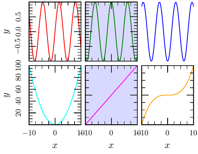
More control on grids

The version 0.14 of ctioga2 introduced several features to ease the drawing of grids. First, it is possible to fill a whole grid by specifying grid:next. Second, all the subplots of the a grid automatically receive the following classes:

• grid-left, grid-right, grid-top and grid-bottom for subplots that are the left, right, top and bottom positions of the grid;
• grid-non-left, grid-non-right, grid-non-top and grid-non-bottom for the complement;
• grid-column-n for the nth column (0-based)
• grid-row-n for the nth row (0-based)
• grid-odd-row, grid-even-row, grid-odd-column and grid-even-column
• grid-i-j for element corresponding to grid:i,j

This can be used for easy styling:

define-axis-style '.grid-non-left axis.left' /decoration=ticks /axis-label-text=' '
define-axis-style '.grid-non-bottom axis.bottom' /decoration=ticks /axis-label-text=' '
define-background-style '.grid-odd-column background' /background-color Blue!15
define-axis-style '.grid-2-0 axis' /decoration=None

setup-grid 3x2 /top=1mm /right=2mm /dy=2mm /dx=2mm
math 
    

inset grid:next
  plot sin(x)
next-inset grid:next
  plot cos(x)
next-inset grid:next
  plot -cos(x)
next-inset grid:next
  plot x**2
next-inset grid:next
  plot 10*x
next-inset grid:next
  plot 0.1*x**3
end

Download command file

Unclipped elements and control of depth

By default, elements drawn within a plot are clipped at the plot boundaries (ie nothing goes out of the plot). However, it is sometimes desirable to have things sticking out of the plot, for instance to draw lines spanning from one plot to another. For that, one can use the /clipped=false options to drawing commands (or plot commands):

math
setup-grid 2x1 /top=1mm
inset grid:0,0
plot 'sin(x)' 
next-inset grid:1,0
ylabel "" 
plot 'x**2'
draw-line /width=5 0,10 -30,10 /color=Red
draw-line /width=5 0,50 -30,50 /color=Blue /clipped=false /depth=5

Download command file

See how the first line, while having the same x extension as the second one, is clipped at plot boundaries. The /depth=5 is here to make sure that the line is drawn in front of the axes (that are drawn between depth 10 and depth 11). If you want something behind the background lines, use a depth over 90. Keep in mind, though, that by construction, TeX text always comes on top whatever depth you use.