ctioga2 the polymorphic plotting program

Filled curves

The original gallery can be found there.

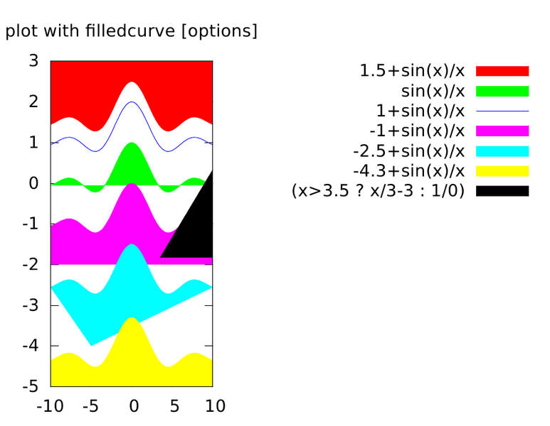
Example: fillcrvs.1

Gnuplot code (download)

set title
set key outside
set title "plot with filledcurve [options]"
plot [-10:10] [-5:3] \
	1.5+sin(x)/x with filledcurve x2, \
	sin(x)/x with filledcurve, \
	1+sin(x)/x with lines, \
	-1+sin(x)/x with filledcurve y1=-2, \
	-2.5+sin(x)/x with filledcurve xy=-5,-4., \
	-4.3+sin(x)/x with filledcurve x1, \
	(x>3.5 ? x/3-3 : 1/0) with filledcurve y2

ctioga2 code (download)

title "plot with filled curves"
color-set gnuplot
auto-legend true
math /xrange=-10:10
yrange -5:3
plot 1.5+sin(x)/x /fill=top
plot sin(x)/x /fill=close
plot 1+sin(x)/x
plot -1+sin(x)/x /fill y=-2
plot -2.5+sin(x)/x /fill xy=-5,-4.
plot -4.3+sin(x)/x /fill bottom
plot "(x>3.5 ? x/3-3 : 1/0)" /fill right

Gnuplot	ctioga2

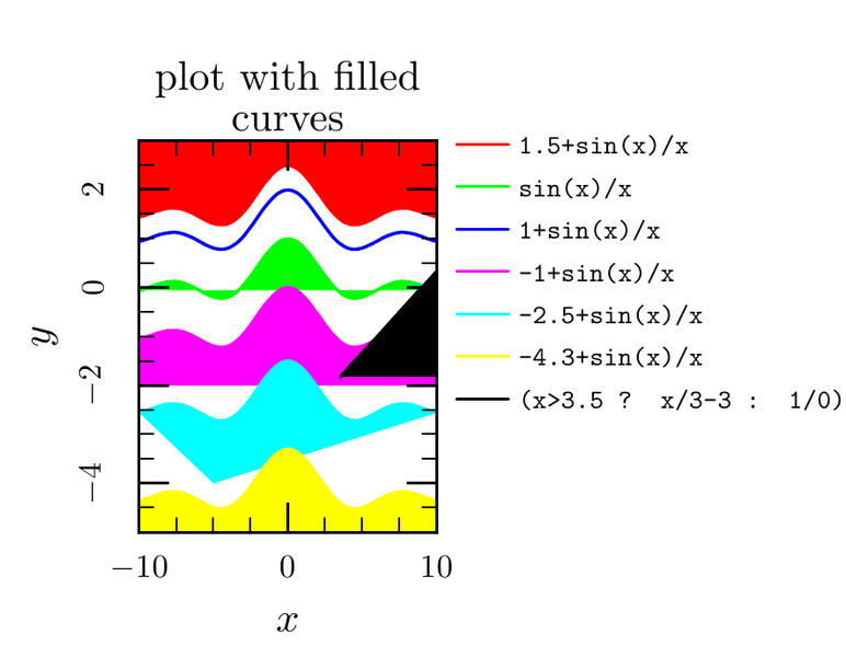Here, we set the color-set to gnuplot to have ctioga2 colors match those of gnuplot, in order to facilitate the comparison between the left and right plots.

Note as well that, as the (x>3.5 ? x/3-3 : 1/0) plot contains spaces, we had to quote it as ctioga2 splits a line into arguments/options at spaces, a bit like the shell.

Example: fillcrvs.2

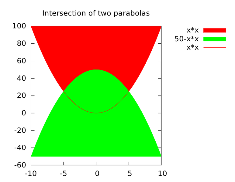
Gnuplot code (download)

set key outside
set title "Intersection of two parabolas"
plot x*x with filledcurves, 50-x*x with filledcurves, x*x with line lt 1

ctioga2 code (download)

auto-legend true
title "Intersection of two parabolas"
math 
plot x*x /fill=top
plot 50-x*x /fill=bottom
plot x*x /color Red

Gnuplot	ctioga2

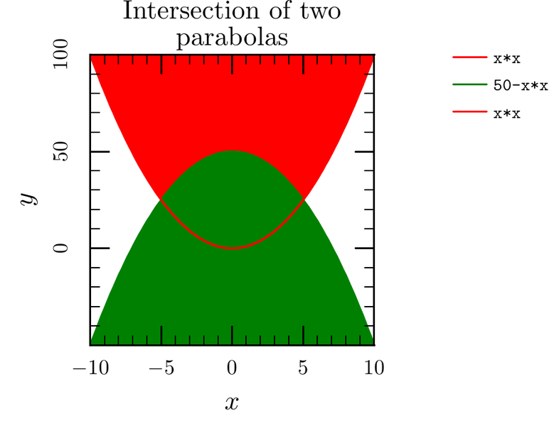Of course, this does not look good, even with ctioga2. It would have been better to take advantage of fill transparency to avoid redrawing the first parabola:

title "Intersection of two parabolas"
math 
plot x*x /fill=top /fill-transparency 0.8 /legend '$x^2$'
plot 50-x*x /fill=bottom /fill-transparency 0.8 /legend '$50 - x^2$'

Download command file

Example: fillcrvs.3

Gnuplot code (download)

set key outside
set grid front
set title "Filled sinus and cosinus curves"
plot 2+sin(x)**2 with filledcurve x1, cos(x)**2 with filledcurve x1

ctioga2 code (download)

title "Filled sinus and cosinus curves"
background-lines left Black /style=Dots
background-lines bottom Black /style=Dots
math
auto-legend true
plot 2+sin(x)**2 /fill=bottom /depth=95
plot cos(x)**2 /fill=bottom /depth=95

Gnuplot	ctioga2

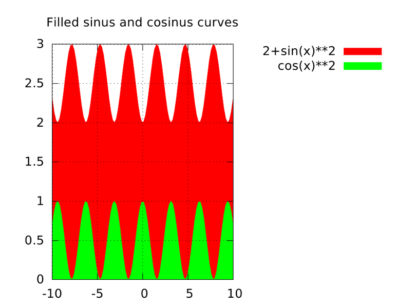We used the option /depth=95 to draw the curves behind the background lines (they are drawn between depth 90 and 91).

Example: fillcrvs.4

Gnuplot code (download)

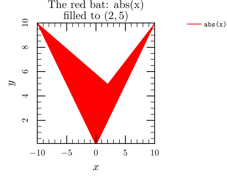
set key outside
set title "The red bat: abs(x) with filledcurve xy=2,5"
plot abs(x) with filledcurve xy=2,5

ctioga2 code (download)

math
auto-legend true
title 'The red bat: abs(x) filled to $(2,5)$'
plot abs(x) /fill xy=2,5

Gnuplot	ctioga2

Example: fillcrvs.5

Gnuplot code (download)

set key outside
set title "Sqrt stripes on filled background"
plot [0:10] [-8:6] \
	-8 with filledcurve x2 lt 15, \
	sqrt(x) with filledcurves y1=-0.5, \
	sqrt(10-x)-4.5 with filledcurves y1=-5.5

ctioga2 code (download)

title "Sqrt stripes on filled background"
math /xrange=0:10
yrange -8:6
auto-legend true
background Blue!40
plot sqrt(x) /fill -0.5
plot sqrt(10-x)-4.5 /fill -5.5

Gnuplot	ctioga2

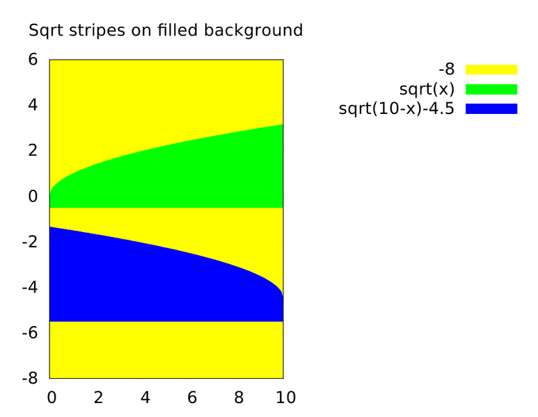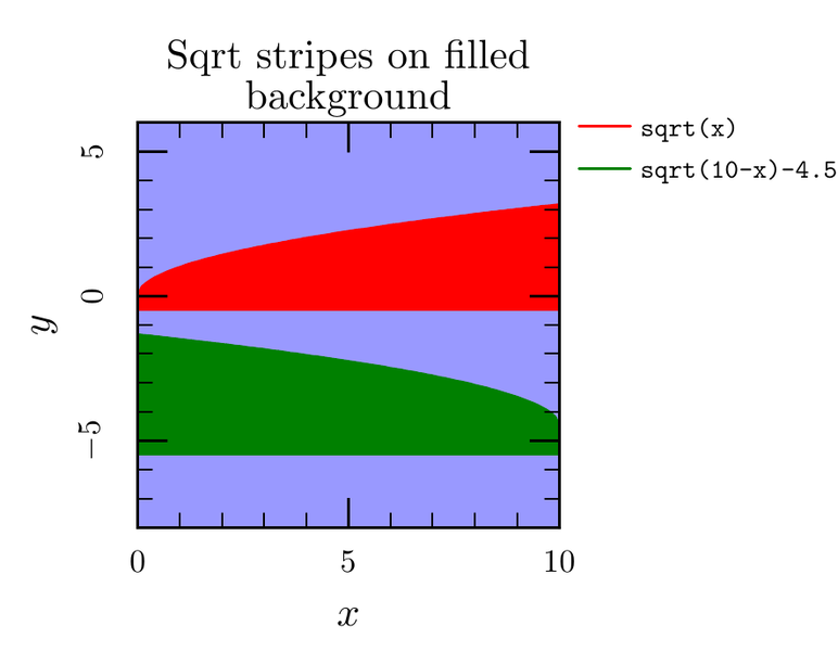Here, it is much smarted to fill the background of the plot rather than to use a constant value. In addition, this ctioga2 plot demonstrates the xcolor-like possibilities to tweak colors: Blue!40 means 40% of Blue mixed with 60% of something else (white by default).

Example: fillcrvs.6

Gnuplot code (download)

set title "Let's smile with parametric filled curves"
set size square
set key off
unset border
unset xtics
unset ytics
set grid
set arrow 1 from -0.1,0.26 to 0.18,-0.17 front size 0.1,40 lt 5 lw 4
set label 1 "gnuplot" at 0,1.2 center front
set label 2 "gnuplot" at 0.02,-0.6 center front
set parametric
set xrange [-1:1]
set yrange [-1:1.6]
plot [t=-pi:pi] \
	sin(t),cos(t) with filledcurve xy=0,0 lt 15,	\
	sin(t)/8-0.5,cos(t)/8+0.4 with filledcurve lt 3,	\
	sin(t)/8+0.5,cos(t)/8+0.4 with filledcurve lt 3,	\
	t/5,abs(t/5)-0.8 with filledcurve xy=0.1,-0.5 lt 1, \
	t/3,1.52-abs(t/pi) with filledcurve xy=0,1.8 lt -1

ctioga2 code (download)

# missing: set size square
title "Let's smile with parametric filled curves"
clear-axes
math /trange=-3.141592:3.141592
xrange -1:1
yrange -1:1.6
plot sin(t):cos(t) /fill xy:0,0 /color Yellow 
plot sin(t)/8-0.5:cos(t)/8+0.4 /fill close /color Blue
plot sin(t)/8+0.5:cos(t)/8+0.4 /fill close /color Blue
plot t/5:(t/5).abs-0.8 /fill xy=0.1,-0.5 /color Red
plot t/3:1.52-(t/3.1415).abs /fill xy=0,1.6 /color Black
draw-arrow -0.1,0.26  0.18,-0.17 /tail-marker None /color '#0F0'
draw-text 0,1.2 "ctioga2" 
draw-text 0.02,-0.6 "ctioga2" 

Gnuplot	ctioga2

Note that one has to change the xy=0,1.8 fill specification to xy=0,1.6 since gnuplot will silently force any point you specify this way to lie within the plot boundaries, which doesn’t make much sense in my eyes (because it makes it very difficult to draw lines that go in a precise direction).

There is no way for now to specify an aspect ratio using ctioga2.

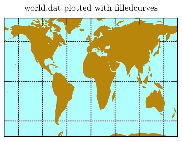
Example: fillcrvs.7

Gnuplot code (download)

set title "world.dat plotted with filledcurves"
set format x ""
set format y ""
set grid layerdefault linewidth 0.5 
set object  1 rect from graph 0, 0 to graph 1, 1 behind fc  rgb "#afffff" fillstyle solid 1.00 border -1
set xrange [ -180.000 : 180.000 ]
set yrange [ -70.0000 : 80.0000 ]
set lmargin  1
plot 'world.dat' with filledcurve notitle fs solid 1.0 lc rgb 'dark-goldenrod'

ctioga2 code (download)

title "world.dat plotted with filledcurves"
no-xlabel
no-ylabel
axis-style left /decoration=major /also-axes=right,top,bottom
background-lines top Black /style Dots
background-lines left Black /style Dots
background "#afffff"
xrange -180:180 
yrange -70:80
text /split=true
plot 'world.dat#1##153' /color DarkGoldenrod /fill close

Gnuplot	ctioga2

Here, we use two esoteric features of ctioga2’s text backend. First, if you turn on the /split option of the text backend (which is also possible using directly the command text-split), ctioga2 will divide the data files into “subsets” separated by blank lines. You select the third subset by adding #3 after the name of the file.

The second esoteric feature is the set expansion. While processing the plot command above, ctioga2 will replace the 1##153 bit by all the numbers from 1 to 153 in succession. The effect is the same as if we had run the plot command on world.dat#1 then on world.dat#2, etc, but it is of course much more compact.

We also took advantage of the /also-axes option to axis-style to use only major ticks for all the axes in one go.

There happen to be exactly 153 bits in the file, but we could have used 1##2000, as ctioga2 just complains when datasets are missing, but doesn’t stop to build the plot.

We use no-xlabel and no-ylabel to disable the display of the X and Y labels. This is different than setting an empty label using {command xlabel} ' ', as the plot does not reserve space for plotting the label, and hence the whole target space is used for the plot.